Superferromagnetism in pinwheel ASI

Here we demonstrate how we used flatspin to replicate the reversal process of pinwheel ASI, as presented by [Li et al., 2019].

“Superferromagnetism and Domain-Wall Topologies in Artificial ‘Pinwheel’ Spin Ice.” ACS Nano 13, no. 2 (January 15, 2019): 2213–22.

A key finding is that when pinwheel ASI is subject to an external field, the angle of the field controls the nature of the reversal process:

1. When the angle is small (equally aligned to both sublattices), reversal happens in a single avalanche.

2. When the angle is large (more aligned to one sublattice), reversal happens in a two-step process where one sublattice switches completely before the other.

Previous attempts at capturing this behavior in a dipole model have proven unfruitful.

The flatspin results are discussed in more detail in our paper [Jensen et al., 2022].

Small angles: 0° and -6°

Fig. 1 and Fig. 2 show the hysteresis loop and snapshots of pinwheel ASI when the angle of the exterernal field is small (\(\theta=0^\circ\) and \(\theta=-6^\circ\)).

Key features:

• Reversal starts at small number of nucleation points, typically close to the edge

• Reversal progresses by domain growth through domain wall movement perpendicular to the direction of the field.

• Reversal is somewhat more ordered for -6° as opposed to 0°.

Fig. 1 Figure 3 (b) from [Li et al., 2019], copyright © American Chemical Society, CC-BY-4.0.

Fig. 2 Figure 3 (a) from [Li et al., 2019], copyright © American Chemical Society, CC-BY-4.0.

Large angles: 30°

Fig. 3 shows the hysteresis loop and snapshots of pinwheel ASI when the angle of the exterernal field \(\theta\) is large.

Key features:

• Reversal process quite different because field now aligned with easy axis of one sublattice

• Ratchetcing behavior yielding a stepped hysteresis loop

• Magnetization constrained to move along 45 degree lines

• Diagonal stripe patterns

Fig. 3 Figure 4 (c) from [Li et al., 2019], copyright © American Chemical Society, CC-BY-4.0.

Size and geometry

Fig. 4 shows a TEM image of the ASI system, where we can deduce the size, shape and lattice spacing:

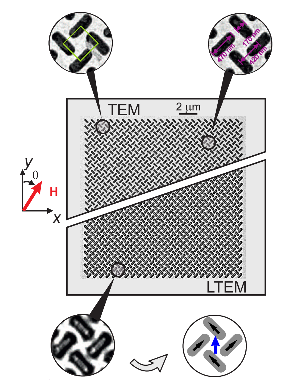
Fig. 4 Figure 1 from [Li et al., 2019], copyright © American Chemical Society, CC-BY-4.0.

In addition, there are some more details from the text [Li et al., 2019]:

Here, we investigate the behavior of a diamond- edge permalloy (Ni 80 Fe 20 ) pinwheel array of two interleaved collinear 25 × 25 sublattices as shown in the in-focus TEM image in the upper half of Figure 1.

Each individual nanomagnetic island is 10 nm thick, 470 nm long, and 170 nm wide, with a center-to- center separation between nearest-neighbor islands of 420 nm, as shown the top right inset to Figure 1.

Note that their geometry differs from the default pinwheel geometry in flatspin:

1. The angles of the first row is -45° (counter-clockwise), as opposed to 45° (clockwise).

2. They use “asymmetric pinwheel edges”

flatspin parameters

We determine simulation parameters based on details from the original paper, mumax simulations for the astroid parameters, as well as some guesswork.

Geometry

From Fig. 4 and the text:

• Size: 25x25

• Edges: asymmetric

• Spin angle: -45° (counter-clockwise)

• Lattice spacing: ~594 nm

  • From Fig. 4, NN distance is 420 nm. That gives a corresponding flatspin lattice spacing of 2 * 420 * cos(45) ~= 594 nm.

External field

• Field angle: -6°, 0° and 30°

  • From Fig. 4, their zero angle is straight up, whereas in flatspin zero is towards the right.

  • Correspoinding flatspin angles are hence 96°, 90° and 60°, respectively.

  • In the following, we refer to flatspin angles using \(\phi\) (phi), i.e., \(\phi=90-\theta\)

• Field strength: approx +/- 300 Oe = +/- 30 mT (from Fig. 3)

Switching parameters

Parameters for switching were estimated from mumax simulations of a single 470x170x10 nm island, subject to an external field at different angles.

• Coercive field \(h_k\) = 0.098

• \(b\) = 0.28

• \(c\) = 1.0

• \(\beta\) = 4.8

• \(\gamma\) = 3.0

We now calculate all the flatspin parameters, and instantiate the model.

from flatspin.model import *
from flatspin.data import *
from flatspin.plotting import plot_vectors, montage_fig
from flatspin.vertices import find_vertices, vertex_pos, vertex_mag

size = (25, 25)
edge = "asymmetric"
spin_angle = -45

# Calculate alpha
Msat = 860e3
nw = 470e-9 # width
nh = 170e-9 # height
nt = 10e-9 # thickness
a = 594e-9 # lattice spacing

M = Msat*nw*nh*nt
mu0 = 1.2566370614e-6
alpha = mu0*M/(4*np.pi*a**3)
alpha = np.round(alpha, 5)

# From hysteresis-470x170x10-roundrect100-sweep-phi-li
hc = 0.098
sw_b = 0.28
sw_beta = 4.8
sw_gamma = 3.0

# Guess disorder
disorder = 0.05

random_seed = 0xdeadbeef

params = dict(
    size=size, edge=edge, spin_angle=spin_angle, lattice_spacing=1,
    hc=hc, alpha=alpha, disorder=disorder,
    switching='sw', sw_b=sw_b, sw_beta=sw_beta, sw_gamma=sw_gamma,
    random_seed=random_seed, use_opencl=1,
)

Visual sanity check

Let’s quickly verify that the resulting flatspin geometry matches the paper (Fig. 4).

model = PinwheelSpinIceDiamond(**params)
model.plot()
plt.axis('off');

Pinwheel units (vertices)

In the paper they consider the magnetization of the “pinwheel units”, similar to vertices from other geometries.

Vertices in pinwheel are a bit different from square. Let’s compare them.

plt.subplot(121)
plt.axis('off')
prms = dict(params)
del prms['spin_angle']
prms.update(size=(4,4))
sq = SquareSpinIceClosed(**prms)
sq.randomize()
sq.plot()
sq.plot_vertices()

plt.subplot(122)
plt.axis('off')
prms = dict(params)
prms.update(size=(4,4))
pw = PinwheelSpinIceDiamond(**prms)
pw.randomize()
pw.plot()
pw.plot_vertices();

Visuals

Here we attempt to replicate the visualization of the pinwheel units, as detailed in Figure S9 (d) from [Li et al., 2019]:

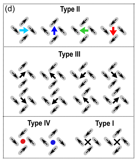
Fig. 5 Figure S9 (d) from [Li et al., 2019], copyright © American Chemical Society, CC-BY-4.0.

# Color map for the magnetization arrows
clist = list('ckkbbkkggkkrrkkc')
clist = ['#00da00' if c == 'g' else c for c in clist]
clist = ['#0800da' if c == 'b' else c for c in clist]
clist = ['#ed0912' if c == 'r' else c for c in clist]
clist = ['#00ccff' if c == 'c' else c for c in clist]

cmap = matplotlib.colors.ListedColormap(clist)
cmap(np.arange(0,1.01,0.125))[:,:3]
rad = np.linspace(0,2*np.pi,360)
gradient = np.vstack((rad, rad))
plt.figure(figsize=(4, .5))
plt.gca().get_yaxis().set_visible(False)
plt.grid(False)
plt.imshow(gradient, aspect='auto', cmap=cmap)
plt.xticks(np.arange(0,360,45));

# Try the color map
model.randomize()
plt.subplot(121)
plt.axis('off')
model.plot()

plt.subplot(122)
plt.axis('off')
model.plot_vertex_mag(cmap='li2019', headwidth=3, headlength=3, headaxislength=2.5);

# Plot vertex magnetization, with added markers for Type I and IV vertices (zero net magnetization)
def plot_vertices(model, markersize=80, ax=None, **kwargs):
    # Find type I and IV vertices
    vertices = model.vertices()
    vertex_types = np.array([model.vertex_type(v) for v in vertices])
    type1, = np.nonzero(vertex_types == 1)
    type4, = np.nonzero(vertex_types == 4)
    spin4 = np.array([model.spin[vertices[v]] for v in type4])
    type4a = type4[[s[0] == 1 for s in spin4]]
    type4b = type4[[s[0] == -1 for s in spin4]]

    if ax is None:
        ax = plt.gca()

    # Plot vertex magnetization
    a1 = model.plot_vertex_mag(
        cmap='li2019', headwidth=3, headlength=3, headaxislength=2.5,
        ax=ax, **kwargs)
    
    # Add markers for Type I and IV vertices
    XY = vertex_pos(model.pos, vertices)
    a2 = ax.scatter(XY[type1, 0], XY[type1, 1],
                    c='black', marker='x', s=markersize, lw=0.05*markersize)
    a3 = ax.scatter(XY[type4a, 0], XY[type4a, 1],
                    c='red', marker='o', s=markersize, edgecolors='none')
    a4 = ax.scatter(XY[type4b, 0], XY[type4b, 1],
                    c='blue', marker='o', s=markersize, edgecolors='none')
    return [a1, a2, a3, a4]

# Test plot_vertices (small system)
plot_vertices(pw)

# Full state in background
pw.plot(alpha=0.2)
plt.axis('off');

plot_vertices(model, 10)
plt.axis('off');

Reversal curves

We are now ready to simulate the reversal process in flatspin. In the code below, we apply an external field at an angle phi. The amplitude of the field is gradually increased from -H to H, and then decreased from H to -H. For each field value, we record the state of the system when one or more spins flipped. In other words, we only record changes in state.

def run_reversal(model, phi, H=0.03, timesteps=101):
    triangle = -sawtooth(np.linspace(0, 2*np.pi, timesteps), 0.5)

    phi_rad = np.deg2rad(phi)
    H = H * triangle

    h_ext = np.column_stack([H * np.cos(phi_rad), H * np.sin(phi_rad)])
    spin = []
    time = []

    model.polarize()
    for i, h_ext_i in enumerate(h_ext):
        model.set_h_ext(h_ext_i)
        steps = model.relax()
        if i == 0 or steps > 0:
            # Store only state when there were spin flips
            time.append(i)
            spin.append(model.spin.copy())

    result = {
        'phi': phi,
        'H': H,
        'time': time,
        'spin': spin,
    }
    
    return result

# Run reversal curves for phi=60 (corresponds to theta=30 in the paper)
result60 = run_reversal(model, 60)

Reversal animation

Animate the state of the system during the different stages of reversal. Note that we only show frames where there have been spin flips.

def animate_reversal(model, phi, H, time, spin):
    fig, ax = plt.subplots()
    fig.subplots_adjust(left=0, right=1, bottom=0.0, top=.9, wspace=0, hspace=0)

    def animate(i):
        t = time[i]
        model.set_spin(spin[i])
        ax.cla()
        ax.set_axis_off()
        ax.set_title(rf"H={H[t]:g} $\theta={90-phi}\degree$")
        plot_vertices(model, markersize=10, ax=ax)

    anim = FuncAnimation(
        fig, animate, init_func=lambda: None,
        frames=len(time), interval=100, blit=False
    )
    plt.close() # Only show the animation
    return HTML(anim.to_jshtml())

Animation: 30°

The animation below shows the full reversal for \(\theta=30^\circ\). Compare with Fig. 3.

animate_reversal(model, **result60)

Once Loop Reflect

Hysteresis loops

Plot H vs M curves. Since we only store changes to state, we need to fill in the gaps where there were no spin flips.

def plot_hysteresis(model, phi, H, time, spin):
    phi_rad = np.deg2rad(phi)
    direction = [np.cos(phi_rad), np.sin(phi_rad)]
    
    # Calculate average magnetization along H
    M = []
    M_H = []
    for s in spin:
        model.set_spin(s)
        mag = model.vectors.sum(axis=0)
        mag_h = mag.dot(direction)
        M.append(mag)
        M_H.append(mag_h)

    M = np.array(M)
    M_H = np.array(M_H)
    M_H /= M_H.max()
    H *= 1000 # mT
    
    # Fill in the gaps
    df = pd.DataFrame({'M_H': M_H}, index=time)
    df = df.reindex(index=np.arange(len(H))).ffill()
    df['H'] = H
    
    plt.plot(df['H'], df['M_H'], '.-')
    plt.grid(True)
    plt.title(rf"$\theta={90-phi}\degree$")
    plt.xlabel("H (mT)")
    plt.ylabel(r"$M_{\parallel H}$")

Hysteresis: 30°

The plot below shows the hysteresis curve for \(\theta=30^\circ\). Compare with Fig. 3.

plot_hysteresis(model, **result60)

Small angles: -6° and 0°

The results above match very well with Fig. 3. Let’s try the smaller angles from Fig. 1 and Fig. 2.

We increase our resolution (timesteps) a bit, since reversal happens much faster at low angles.

result96 = run_reversal(model, 96, timesteps=501)
result90 = run_reversal(model, 90, timesteps=501)

Below we produce the reversal animations and hysteresis curves for the two small angles. Compare with Fig. 1 and Fig. 2.

animate_reversal(model, **result90)

Once Loop Reflect

plot_hysteresis(model, **result90)

animate_reversal(model, **result96)

Once Loop Reflect

plot_hysteresis(model, **result96)

Budrikis switching

In [Li et al., 2019] they also attempt to reproduce the results using a dipole model:

However, it is worth noting that despite extensive efforts to replicate the precise details of the magnetization, this model does not adequately capture the richness of the behavior discussed in the following sections.

A crucial difference between their dipole model and flatspin, is that their model employ a much simpler switching criteria, only considering the component of the field parallel to the easy axis of each magnet.

In flatspin, this simpler switching criteria is available as “Budrikis switching”, named after [Budrikis, 2012]. Let’s examine how Budrikis switching affects the reversal process. We start with \(\theta=0^\circ\).

prms = dict(params)
prms['switching'] = "budrikis"
prms['hc'] = 0.013 # match hysteresis @ 90 degrees
model_budrikis = PinwheelSpinIceDiamond(**prms)
result90_budrikis = run_reversal(model_budrikis, 90, -0.03, 501)

animate_reversal(model_budrikis, **result90_budrikis)

Once Loop Reflect

plot_hysteresis(model_budrikis, **result90_budrikis)

Although we are able to get a good match for the hysteresis loop (compare with Fig. 1), the animation reveals a very different reversal process, with apparent domains in all directions (not just up/down).

Next, we try \(\theta=-6^\circ\).

result96_budrikis = run_reversal(model_budrikis, 96, -0.03, 501)

animate_reversal(model_budrikis, **result96_budrikis)

Once Loop Reflect

plot_hysteresis(model_budrikis, **result96_budrikis)

At \(\theta=-6^\circ\) we see the hysteresis loop has changed significantly. We now have a two-dimensional avalanche, instead of one-dimensional (compare with Fig. 2).

Finally, try \(\theta=30^\circ\).

result60_budrikis = run_reversal(model_budrikis, 60, -0.06, 501)

animate_reversal(model_budrikis, **result60_budrikis)

Once Loop Reflect

plot_hysteresis(model_budrikis, **result60_budrikis)

At \(\theta=30^\circ\), we have to double the strength of the external field to obtain full reversal. Although the animation is similar, the hysteresis loop is very different from Fig. 3.

Reproduce the figures

Finally, we reproduce the figures from the paper more exactly. Instead of running the simulations in this notebook, we use the command-line tools of flatspin to run the experiments. This has the advantage of storing the results in as a dataset, should we wish to perform more analysis later.

# Read the dataset
dataset = Dataset.read('/data/flatspin/pw-li-sweep-phi-new4')

# Print the command used to generate the results
# You can run this command yourself to reproduce the dataset
cmd = dataset.info['command'].split(" ")
cmd[0] = basename(cmd[0])
cmd[-1] = basename(cmd[-1])
print(" ".join(cmd))

flatspin-run-sweep -r dist -m PinwheelSpinIceDiamond -e triangle -p 'size=(25, 25)' -p edge=asymmetric -p spin_angle=-45 -p lattice_spacing=1 -p hc=0.098 -p alpha=0.00033 -p disorder=0.05 -p switching=sw -p sw_b=0.28 -p sw_beta=4.8 -p sw_gamma=3.0 -p use_opencl=1 -p H=-0.03 -p periods=1 -s 'phi=[90, 96, 60]' -p timesteps=10000 -p spp=10000 -p random_seed=3735928559 -o pw-li-sweep-phi-new4

# For inclusion in the Flatspin2022 paper, we enabled latex for the plots
# Use latex
#plt.rcParams.update({
#    "text.usetex": True,
#    "text.latex.preamble": r"\usepackage{gensymb}",
#})

# Function for plotting hysteresis from the dataset
def plot_data_hysteresis(dataset, **kwargs):
    df = read_table(dataset.tablefile('mag'), index_col='t')
    UV = np.array(df)
    UV = UV.reshape((UV.shape[0], -1, 2))
    
    df = read_table(dataset.tablefile('h_ext'), index_col='t')
    h_ext = np.array(df)
    h_ext = h_ext.reshape((-1, 2))
    
    pos, angle = read_geometry(dataset.tablefile('geometry'))

    phi = dataset.row(0)['phi']
    theta = np.deg2rad(phi)
    direction = [np.cos(theta), np.sin(theta)]
    
    H = h_ext.dot(direction)
    M = UV.sum(axis=1)
    M_H = M.dot(direction)
    M_H /= M_H.max()
    
    plt.grid(True)
    plt.title(rf'$\theta={90-phi}\degree$')
    plt.plot(H * 10000, M_H, '.-', **kwargs)
    plt.xlabel("Magnetic Field (Oe)")
    plt.ylabel(r"$M / M_{\mathrm{S}}$")

# Function for plotting the vertex magnetization from the dataset
def plot_data_vertices(dataset, t=[0], markersize=1):
    df = read_table(dataset.tablefile('mag'), index_col='t')
    UV = np.array(df)
    UV = UV.reshape((UV.shape[0], -1, 2))
    UV = UV[t]
    
    df = read_table(dataset.tablefile('spin'), index_col='t')
    spin = np.array(df)
    spin = spin[t]
    
    pos, angle = read_geometry(dataset.tablefile('geometry'))

    phi = dataset.row(0)['phi']
    theta = np.deg2rad(phi)
    direction = [np.cos(theta), np.sin(theta)]
    
    # Map the vectors on the native grid
    grid = Grid(pos)

    vi, vj, vertices = find_vertices(grid, pos, angle, (3, 3))

    XY = pos
    XY = vertex_pos(pos, vertices)
    UV = np.array([vertex_mag(UVi, vertices) for UVi in UV])
    UV /= 2
    
    for UVi, spini in zip(UV, spin):
        plt.axis('off')
        plot_vectors(XY, UVi, cmap='li2019', headwidth=4, headlength=4, headaxislength=3.5)
        
        vertex_types = np.array([vertex_type(spini[v], pos[v], angle[v]) for v in vertices])
        type1, = np.nonzero(vertex_types == 1)
        type4, = np.nonzero(vertex_types == 4)
        spin4 = [spini[vertices[v]] for v in type4]
        type4a = type4[[s[0] == 1 for s in spin4]]
        type4b = type4[[s[0] == -1 for s in spin4]]
        
        plt.scatter(XY[type1, 0], XY[type1, 1], c='black', marker='x', s=markersize, lw=0.2*markersize)
        plt.scatter(XY[type4a, 0], XY[type4a, 1], c='red', marker='o', s=markersize, edgecolors='none')
        plt.scatter(XY[type4b, 0], XY[type4b, 1], c='blue', marker='o', s=markersize, edgecolors='none')

# Make a figure similar to Li2019
figsize=(3,3)
def make_fig():
    fig = plt.figure(figsize=figsize)
    gs = fig.add_gridspec(3, 3, hspace=0, wspace=0, top=1, bottom=0, left=0, right=1)
    # ugh...
    sgs = gs[0:2, 0:2].subgridspec(3, 3, height_ratios=[5-2.5, 80, 20-2.5], width_ratios=[25-2.5, 70+5, 5-2.5])
    ax1 = fig.add_subplot(sgs[1,1])
    #ax1 = fig.add_subplot(gs[0:2,0:2])
    ax1.set_xlabel('xlab')
    ax1.set_ylabel('ylab')
    ax1.set_title('title')
    
    ax2 = fig.add_subplot(gs[0, 2])
    ax3 = fig.add_subplot(gs[1, 2])
    ax4 = fig.add_subplot(gs[2, 2])
    ax5 = fig.add_subplot(gs[2, 1])
    ax6 = fig.add_subplot(gs[2, 0])
    
    return ax1, (ax2, ax3, ax4, ax5, ax6)

make_fig();

def plot_data_hyst_verts(dataset, hyst_color, times):
    hyst_ax, vert_axes = make_fig()
    
    plt.sca(hyst_ax)
    plot_data_hysteresis(dataset, color=hyst_color)
    hyst_ax.xaxis.set_major_locator(mpl.ticker.MultipleLocator(200))
    hyst_ax.yaxis.set_major_locator(mpl.ticker.MultipleLocator(1))

    for t, ax in zip(times, vert_axes):
        plt.sca(ax)
        #plt.title(str(t))
        plot_data_vertices(dataset, [t])

phi=90
ds = dataset.filter(phi=phi)
times = [1418, 1446, 1453, 1471, 1493]
plot_data_hyst_verts(ds, '#000080', times)

phi=96
ds = dataset.filter(phi=phi)
times = [1449, 1470, 1475, 1482, 1558]
plot_data_hyst_verts(ds, '#7F0000', times)

phi=60
ds = dataset.filter(phi=phi)
times = [1594, 1649, 1806, 2299, 2470]
plot_data_hyst_verts(ds, '#FF8000', times)