Command-line tools#

In addition to the Python API, flatspin comes with a set of powerful command-line tools. These are installed automatically as part of the flatspin package.

If you find that the commands are not available in your shell automatically, you may need to modify your PATH variable. The location of the command-line tools varies based on the operating system and installation method.

If you installed flatspin in your home directory (using pip install --user):

export PATH=$PATH:$HOME/.local/bin

The command-line tools can be understood from the flatspin architecture:

flatspin architecture

In the figure, the arrows indicate data flow between the components:

The input encoder translates input to a field protocol (series of external fields).
The runner perturbs the ASI model according to the field protocol, and saves the results.
The results are stored in a dataset
Analysis tools read and process the dataset.

Note

A good understanding of the concepts introduced in the rest of this User Guide is beneficial to effectively use the command-line tools.

Running simulations#

flatspin simulations can be run directly from the command line, using the commands flatspin-run and flatspin-run-sweep. These tools were designed to be flexible enough to allow for a range of different simulation scenarios.

Some notable features include:

Results are stored in the standard dataset format for later analysis.
All simulation parameters can be specified from the command-line.
Input encoders are used to define the external field.
Parameter sweeps can be defined to run many simulations in one go.
Simulations may be run in parallel on a compute cluster.

`flatspin-run`#

To run a single flatspin simulation, use flatspin-run.

Let us start with a simple example:

flatspin-run -o /tmp/flatspin/myrun -m SquareSpinIceClosed \
             -e Triangle -p H=100e-3 -p phase=-90 -p phi=30 -p periods=1

/builds/flatspin/flatspin/.tox/docs/lib/python3.10/site-packages/flatspin/runner.py:90: UserWarning: Ignoring unknown parameters: outdir

  warnings.warn("Ignoring unknown parameters: " + unknown_params)

Run 1/1: outdir=SquareSpinIceClosed.npz

Completed 80 steps in 0:00:00.340047

The -o/--basepath argument specifies the directory where simulation results will be stored as a dataset. This directory should not already exist, and will be automatically created by flatspin-run.

The -m/--model argument refers to the model class to use. You may also specify your own model class by providing the full module path, e.g., -m mymodels.MySpinIce.

The -e/--encoder argument specifies the input encoder to use for defining the field protocol. In the example, the Triangle encoder is used which results in a linear ramped external field. For a list of available encoders, see flatspin-run --list-encoders. You may also specify your own encoder class by providing the full module path, e.g., -e myencoders.MyEncoder.

The -p/--param arguments are parameters to the model, the runner and the encoder:

-p H=100e-3 sets the amplitude of the external field to 100 mT
-p phase=-90 sets the phase of the triangle wave to -90°
-p phi=30 sets the angle of the external field to 30°
-p periods=1 sets the number of field cycles to 1

For a list of available parameters, append --list-params to the flatspin-run command.

The runner#

The runner is responsible for running the simulation. In simplified pseudocode, the runner does the following:

model = ModelClass(model_params)
encoder = EncoderClass(encoder_params)
h_ext = encoder(input)
for h in h_ext:
    model.set_h_ext(h)
    model.relax()
    if should_sample:
        record current state of the model
save recorded states as tables in the dataset

As you can see, the external field is what drives the simulation. Each value of h_ext is immediately followed by a call to model.relax(), which flips any spins in response to the new field value.

Parameters#

The parameters passed by the -p/--param arguments are consumed in the following order:

The model class (passed to the constructor)
The runner (passed to flatspin.runner.run())
The encoder class (passed to Encoder.set_params()

It is assumed that there is never overlap between the parameter names for the model, runner and encoders.

For a list of available parameters, append --list-params to the flatspin-run command. Documentation for each parameter can be found in the model class, the runner and the corresponding encoder class flatspin.encoder.

Parameter values are evaluated as Python code (using eval). Values may use numpy code, e.g., -p param=np.random.rand(). Some additional utility functions are also available, see flatspin.cmdline.param_globals.

Input#

The input to the encoder may provided in a few different ways:

Passed directly as an array: -p input=[0.3, 0.5, 1.0]
Created indirectly: -p periods=P which is short-hand for -p input=[1]*P
Loaded from file: -p input=myinput.csv which is read with read_table(). To select a specific column to use: -p input_key=column_name.

Selecting the sample rate: `spp` and `timesteps`#

The encoder may produce many h_ext values for each input value. The number of h_ext values is typically controlled by the timesteps encoder parameter. For example, the Triangle encoder uses timesteps=100 by default, meaning there will be 100 h_ext field values per input value.

The spp runner parameter determines how often the state of the model should be sampled (and saved). The parameter name spp is an abbreviation for samples per period, and specifies the number samples per input period. In the Triangle example, we can use -p spp=100 to sample the model state after every h_ext value, or -p spp=50 to sample every other h_ext value, or -p spp=1 to sample once for each input value (sampled at the beginning of the input).

Some care must be taken when choosing spp such that it is compatible with timesteps. It is the users responsibility to ensure that spp evenly divides timesteps (a warning is generated if it does not).

Time-varying parameters#

Some model parameters may also be modified dynamically over time. Time-varying parameters can be defined by adding a _t suffix to the parameter name, for example:

flatspin-run ... -p temperature_t='[400, 350, 300]'

will create a time-varying temperature with three values. The length of all time-varying parameters must match the length of the input.

Currently, the following time-varying parameters are supported: alpha_t, hc_t, m_therm_t, spin_t, temperature_t, therm_timescale_t, threshold_t The external field must be created using the input encoder, i.e., h_ext_t is not allowed.

`flatspin-run-sweep`#

Often we wish to explore how an ASI changes behavior under different parameters. Parameter sweeps is a simple and effective way to systematically explore the effect of one or multiple parameters.

flatspin-run-sweep accepts a list of parameters to sweep, and runs a series of flatspin simulations using the given parameter values. Continuing our simple example, we sweep the field strength H:

flatspin-run-sweep -o /tmp/flatspin/mysweep -m SquareSpinIceClosed \
                   -e Triangle -p phase=-90 -phi=30 -p periods=1 \
                   -s 'H=[80e-3, 84e-3, 88e-3, 92e-3]'

/builds/flatspin/flatspin/.tox/docs/lib/python3.10/site-packages/flatspin/runner.py:90: UserWarning: Ignoring unknown parameters: outdir

  warnings.warn("Ignoring unknown parameters: " + unknown_params)

/builds/flatspin/flatspin/.tox/docs/lib/python3.10/site-packages/flatspin/runner.py:90: UserWarning: Ignoring unknown parameters: outdir

  warnings.warn("Ignoring unknown parameters: " + unknown_params)

/builds/flatspin/flatspin/.tox/docs/lib/python3.10/site-packages/flatspin/runner.py:90: UserWarning: Ignoring unknown parameters: outdir

  warnings.warn("Ignoring unknown parameters: " + unknown_params)

/builds/flatspin/flatspin/.tox/docs/lib/python3.10/site-packages/flatspin/runner.py:90: UserWarning: Ignoring unknown parameters: outdir

  warnings.warn("Ignoring unknown parameters: " + unknown_params)

Starting sweep with 4 runs

Run 1/4: H=0.08 outdir=SquareSpinIceClosed.000000.npz

Completed 24 steps in 0:00:00.286613

Run 2/4: H=0.084 outdir=SquareSpinIceClosed.000001.npz

Completed 38 steps in 0:00:00.297268

Run 3/4: H=0.088 outdir=SquareSpinIceClosed.000002.npz

Completed 44 steps in 0:00:00.309533

Run 4/4: H=0.092 outdir=SquareSpinIceClosed.000003.npz

Completed 80 steps in 0:00:00.348458

The -s/--sweep argument in the above command specifies a sweep of the parameter H with a list of values ranging from 80 mT to 92 mT.

Note how the invocation of flatspin-run-sweep is identical to flatspin-run, with the addition of -s/--sweep.

Multiple parameters may be swept by providing multiple -s/--sweep arguments, in which case all combinations of parameter values will be swept.

For example, the command:

flatspin-run-sweep ... -s 'phi=[0, 30, 45]' -s 'H=[80e-3, 84e-3, 88e-3, 92e-3]'

would sweep the two parameters phi and H, starting with phi=0, H=80e-3, then phi=0, H=84e-3, and so on until finally phi=45, H=92e-3 is reached. The above sweep would result in a total of 12 flatspin runs.

In addition, each run may be repeated N times with -n/--repeat N. This is useful when simulating stochastic systems, e.g., with disorder or thermal fields enabled.

Distributed running#

As the number of parameters grow, it may be beneficial to distribute the simulations onto a compute cluster to run them in parallel. Distributed running is supported both by flatspin-run and flatspin-run-sweep with the -r dist argument.

flatspin uses SLURM to submit cluster jobs. Currently you need to edit the file flatspin.slurm.sh to configure flatspin for your particular cluster. Other job schedulers should be possible with minimal code changes.

Analysis tools#

A set of analysis tools are included in flatspin, which all operate on datasets such as those produced by flatspin-run and flatspin-run-sweep.

`flatspin-inspect`#

flatspin-inspect is a handy tool to quickly get an overview of the contents of a dataset.

For example, let us have a look at the sweep we created above:

flatspin-inspect -b /tmp/flatspin/mysweep -l

Dataset: mysweep

params:

 alpha=0.001

 astroid_resolution=1801

 attempt_freq=1000000000.0

 disorder=0

 edge=symmetric

 encoder=flatspin.encoder.Triangle

 flip_mode=max

H=1

 H0=0

 h_ext=(0, 0)

 hc=0.2

 init=polarized

 input=1

 input_key=None

 lattice_spacing=1

 m_therm=7.567999999999999e-17

 neighbor_distance=1

 opencl_device=0

 opencl_platform=0

 periods=1

 phase=-90

 phi=30

 random_prob=0.5

 random_seed=0

 size=(4, 4)

 spin_axis=None

 spp=100

 sw_b=0.41

 sw_beta=1.5

 sw_c=1

 sw_gamma=3.9

 switching=sw

 temperature=0

 therm_timescale=1

 timesteps=100

 use_cuda=False

 use_opencl=False

info:

 command: /builds/flatspin/flatspin/.tox/docs/bin/flatspin-run-sweep -o /tmp/flatspin/mysweep -m SquareSpinIceClosed -e Triangle -p phase=-90 -p phi=30 -p periods=1 -s 'H=[80e-3, 84e-3, 88e-3, 92e-3]'

 data_format: npz

 model: flatspin.model.SquareSpinIceClosed

 model_name: SquareSpinIceClosed

 version: 2.3

index:

       H                          outdir

0  0.080  SquareSpinIceClosed.000000.npz

1  0.084  SquareSpinIceClosed.000001.npz

2  0.088  SquareSpinIceClosed.000002.npz

3  0.092  SquareSpinIceClosed.000003.npz

The output of flatspin-inspect -l consists of three parts:

Parameter listing params: A list of all the parameters used in the run. Notice how this listing contains parameters that were not specified in the flatspin-run-sweep command. These parameters record the default values at the dataset creation time.
Information info: Miscellaneous information about the run, including the full flatspin-run-sweep command.
The index of the runs in the dataset: the index contains one column for each swept parameter.

Tip

If the -b/--datapath argument is omitted, the flatspin analysis tools will look for a dataset in the current working directory.

Tables included in a run#

Let us have a look at what tables are available within each run:

flatspin-inspect -b /tmp/flatspin/mysweep

[0] H=0.08 outdir=SquareSpinIceClosed.000000.npz:

    tables (11): energy[t], geometry, h_ext[t], hc, init, input[t], mag[t], params, spin[t], stats, steps[t]

[1] H=0.084 outdir=SquareSpinIceClosed.000001.npz:

    tables (11): energy[t], geometry, h_ext[t], hc, init, input[t], mag[t], params, spin[t], stats, steps[t]

[2] H=0.088 outdir=SquareSpinIceClosed.000002.npz:

    tables (11): energy[t], geometry, h_ext[t], hc, init, input[t], mag[t], params, spin[t], stats, steps[t]

[3] H=0.092 outdir=SquareSpinIceClosed.000003.npz:

    tables (11): energy[t], geometry, h_ext[t], hc, init, input[t], mag[t], params, spin[t], stats, steps[t]

From the output above, we can see that each run in the dataset contains quite a few tables. Tables marked with a [t] contain time-dependent data. Below is a short description of the tables, with references to the releated model attributes or methods.

Table	Description
`energy`	Energy over time
`geometry`	Position and angle of each spin
`h_ext`	External field over time
`h_therm`	Thermal field over time (if `temperature > 0`)
`hc`	Coercive fields of each spin
`init`	Initial state of each spin
`input`	Input over time
`mag`	Magnetization vectors over time
`params`	Parameter listing
`params_t`	Time-varying parameters over time (if any)
`spin`	Spin state over time
`stats`	Run statistics
`steps`	Cumulative number of steps over time

Subset and filter#

Just like the flatspin dataset API, we can select a subset of the dataset with -i/--subset or -s/--filter:

flatspin-inspect -b /tmp/flatspin/mysweep -i 1:2

[1] H=0.084 outdir=SquareSpinIceClosed.000001.npz:

    tables (11): energy[t], geometry, h_ext[t], hc, init, input[t], mag[t], params, spin[t], stats, steps[t]

[2] H=0.088 outdir=SquareSpinIceClosed.000002.npz:

    tables (11): energy[t], geometry, h_ext[t], hc, init, input[t], mag[t], params, spin[t], stats, steps[t]

flatspin-inspect -b /tmp/flatspin/mysweep -s H=0.084

[1] H=0.084 outdir=SquareSpinIceClosed.000001.npz:

    tables (11): energy[t], geometry, h_ext[t], hc, init, input[t], mag[t], params, spin[t], stats, steps[t]

In fact, all the flatspin analysis tools support a common set of command-line options, such as -i/--subset, -s/--filter and -l/--list.

`flatspin-plot`#

For quickly plotting data from a dataset, flatspin-plot is your friend.

Let us plot the external field over time from the myrun dataset created earlier:

flatspin-plot -b /tmp/flatspin/myrun -x t -y h_ext

Similarly, we can plot data from multiple runs:

flatspin-plot -b /tmp/flatspin/mysweep -k H -x t -y h_ext

Plot everything from a given table with -g/--table:

flatspin-plot -b /tmp/flatspin/myrun -x t -g energy

Rudimentary functions are also supported, e.g., to sum of all the spins over time:

flatspin-plot -b /tmp/flatspin/mysweep -k H -x t -y 's=sum(spin*)'

… or the same data plotted as a heatmap:

flatspin-plot -b /tmp/flatspin/mysweep -k H -x t -z 's=sum(spin*)'

Arbitrary columns may be used on the x-axis:

flatspin-plot -b /tmp/flatspin/myrun -x 'mx=sum(mag*x)' -y 'my=sum(mag*y)'

See flatspin-plot --help for a full list of options.

`flatspin-vectors`#

Use flatspin-vectors to animate spin vectors over time. The time steps to include can be limited using -t start:stop:step. In the command below we include all time steps, and draw vectors as arrows.

flatspin-vectors -b /tmp/flatspin/myrun -t ::1 --style=arrow

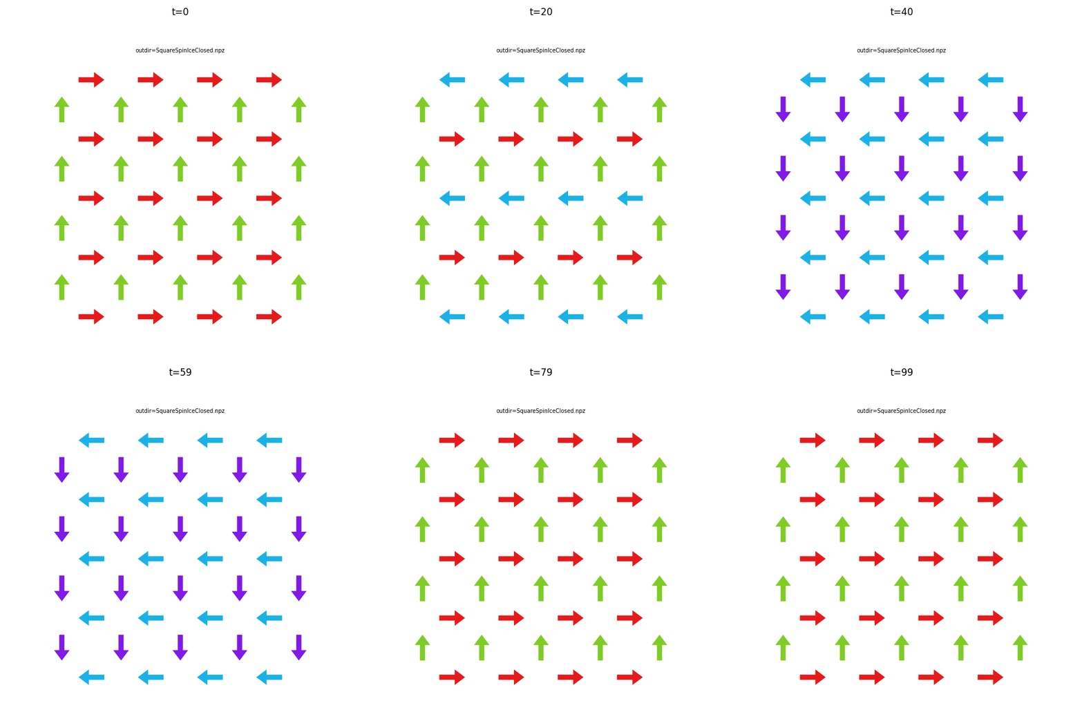
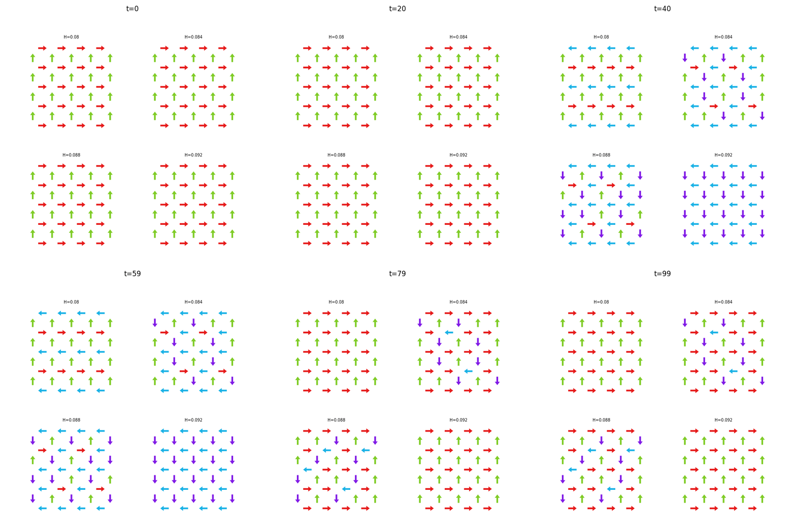
It is often useful to compare results from multiple runs. When the dataset contains multiple runs, flatspin-vectors animates them side by side in a montage:

flatspin-vectors -b /tmp/flatspin/mysweep -t ::1 --style=arrow

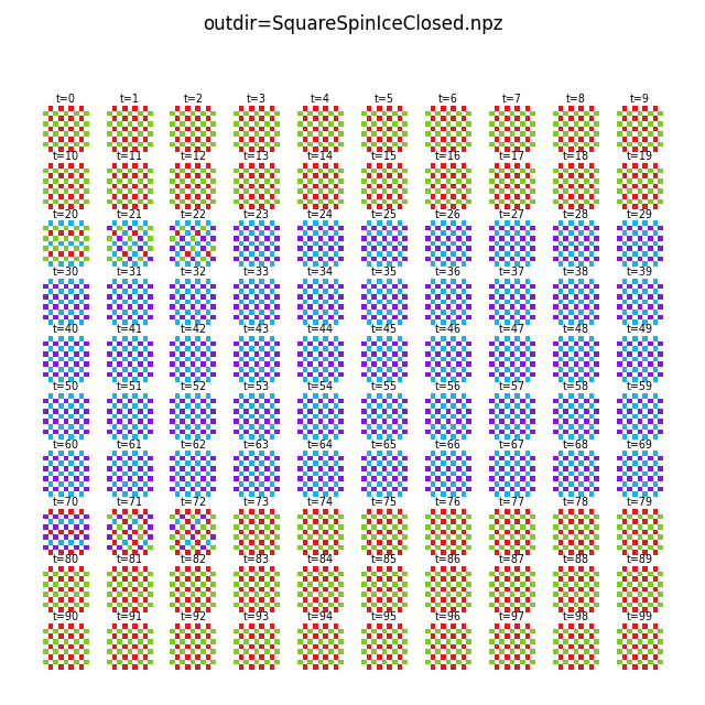
It is also possible to create a montage over time, where each image corresponds to the same run at different points in time. Montage over time is enabled with -a/--animate-dataset. When the images become small, it is a good idea to use the default --style=image, which results in a grid based visualization instead.

flatspin-vectors -b /tmp/flatspin/myrun -t ::1 -a

By default, flatspin-vectors animates the spin vectors, but other quantities can be specified with -q/--quantity:

flatspin-vectors -b /tmp/flatspin/myrun -t ::1 --style=arrow -q h_ext

Apply a grid#

A grid may be applied to the vectors to produce an aggregate view with -g/--grid. Below we apply a 2x2 grid and sum the vectors in each grid cell:

flatspin-vectors -b /tmp/flatspin/myrun -t ::1 -a -g 2

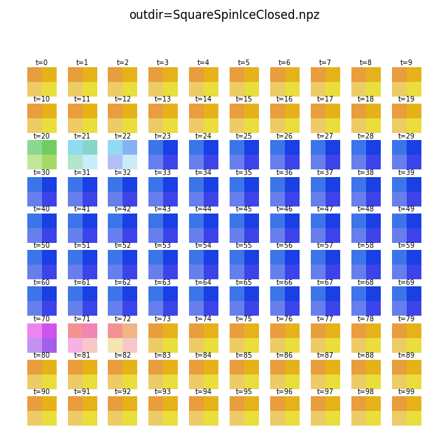
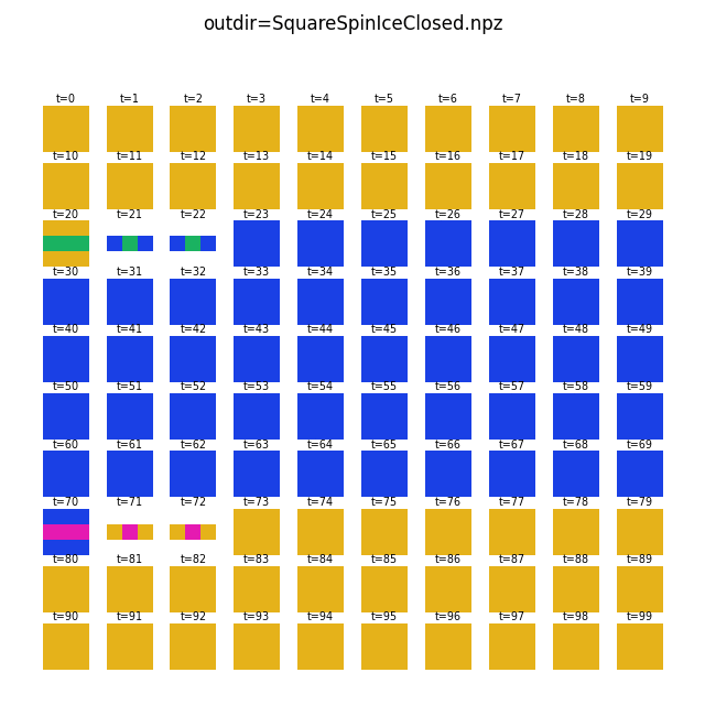
The different color shades in the images above are caused by each grid cell having a different number of spins. For the square closed geometry, we can obtain vertex magnetization by first cropping away the spins at the edges (-c/--crop 1), and then apply a sliding 3x3 window with a step size of 2 (-w/--window 3 2):

flatspin-vectors -b /tmp/flatspin/myrun -t ::1 -a -c 1 -w 3 2

For other geometries, the above windowing trick may not be applicable to find vertices. The flatspin-vertices tool is similar to flatspin-vectors, but employs vertex detection to correctly visualize vertex magnetization for all the included geometries.

Other tools#

In this guide, we have introduced some of the most commonly used command-line tools in flatspin. Several other tools are included, available with the flatspin- prefix. For a full list of command-line tools, see Command-line reference.

Command-line tools

Contents

Command-line tools#

Running simulations#

flatspin-run#

The runner#

Parameters#

Input#

Selecting the sample rate: spp and timesteps#

Time-varying parameters#

flatspin-run-sweep#

Distributed running#

Analysis tools#

flatspin-inspect#

Tables included in a run#

Subset and filter#

flatspin-plot#

flatspin-vectors#

Apply a grid#

Other tools#

`flatspin-run`#

Selecting the sample rate: `spp` and `timesteps`#

`flatspin-run-sweep`#

`flatspin-inspect`#

`flatspin-plot`#

`flatspin-vectors`#